
Reading time: ~22 minutes
If you have ever tried to deploy a 7B+ parameter language model in production, you already know the problem. The model is brilliant, but it is dense — every parameter fires for every token. The FFN layers alone own two-thirds of the parameters and two-thirds of the inference cost. So you stare at your GPU bill and wonder: do I really need every neuron active for every single token?
The Mixture-of-Experts (MoE) answer is no. Route each token to a small subset of expert sub-networks, keep the total parameter count high, but activate only a fraction per token. Qwen3-30B-A3B has 30.5B parameters but activates only 3.3B per token — a 9× effective speedup.
The catch? Training MoEs from scratch is brutal. They are unstable, data-hungry, and need trillions of tokens to converge. Which is why the industry has converged on a smarter idea: take a dense model you already paid to pretrain, and convert it into a sparse MoE. This is called MoEfication.
The bottleneck of MoEfication is a deceptively simple question:
Which neurons go into which expert?
For a 7B model with d_ffn ≈ 14,000, there are roughly 14,000! / (128!)^112 balanced partitions. That number has more digits than atoms in the universe. Prior work fell back to heuristics: random splits, weight clustering, k-means on activations.
DOT-MoE (Bamba, Chavan, Thakur, Teig, Gupta — ICML 2026) throws out the heuristics and reframes the question as something elegant: a balanced optimal transport problem. Solve it differentiably with Sinkhorn iterations, plug in a straight-through estimator, and you get an assignment that is learned end-to-end against the actual output of the dense model — not against some proxy.
The result: 90% of dense performance retained at 50% active parameters, in under 3 hours on 8× H100, beating every structured pruning, semi-structured pruning, and dense-to-MoE baseline the authors could find.
In this article, we are going to understand DOT-MoE from first principles — the math, the architecture, the algorithm, the dry run, the experimental results, and why this approach quietly dominates everything that came before it.
Let's start with what a Transformer FFN actually computes. For a hidden state x ∈ ℝ^d:

Where W_gate, W_up ∈ ℝ^{d×d_ffn}, W_down ∈ ℝ^{d_ffn×d}, σ is an activation like SiLU, and ⊙ is element-wise multiplication.
The key observation: d_ffn is huge. For LLaMA-3-8B it is 14,336. For Qwen2.5-7B it is 18,944. Every single token pays the full O(d_ffn) cost — even though many of those neurons fire weakly and redundantly. The dense activation pattern is the fundamental inefficiency.
Here is the thing: a typical FFN has roughly two-thirds of all model parameters. If you could make the FFN sparse without losing the model's intelligence, you would cut inference cost dramatically.
That is exactly what MoE does.
MoE solves the dense-activation problem by routing each token to a small subset of k experts (out of E), so per-token cost drops to O(k · d_ffn / E). The routing is done by a small linear layer:

Qwen3-30B-A3B activates only 3.3B of 30.5B params per token. Mixtral 8x7B activates 2 of 8 experts per token. The inference speedup is real.
But training an MoE from scratch is a different beast:
So if you already have a 7B dense model that cost millions of dollars to pretrain, asking you to re-pretrain it as an MoE feels insulting. There has to be a better way.
There is.
The cheap alternative is MoEfication (Zhang et al., 2022): take your existing dense checkpoint, partition its FFN's d_ffn neurons into E disjoint expert sub-networks of s = d_ffn / E neurons each, and train a router to pick top-k experts per token. Total parameters preserved; per-token activation reduced.
The hard question, again: which neurons go into which expert?
The combinatorial space is breathtaking:

For LLaMA-3-8B with d_ffn=14336, E=112, s=128 — this number is astronomically large. You cannot brute-force it. Prior work fell back to heuristics:
| Method | Assignment Strategy |
|---|---|
| LLaMA-MoE | Random partition + heavy retraining |
| LTE / MoEfication | Cluster neurons by similarity of W_gate / W_up weights |
| LLaMA-MoE-v2 | Cluster by activation + gradient importance |
| CMoE | Balanced k-means on intermediate activations H |
All of these share a fundamental flaw, and it is worth pausing to really understand it.
Look again at the FFN equation:
FFN(x) = H · W_down
The output of the FFN depends on the interaction between the intermediate activations H and the down-projection weights W_down. Now consider what each prior method does:
W_gate columns look similar. But it ignores how those neurons' activations H will actually be used downstream.H. But two neurons can co-fire and have W_down columns that point in opposite directions — they cancel out. Grouping them produces an expert that is internally fighting itself.Every prior method optimizes a proxy for the output — never the output itself.
The DOT-MoE authors empirically validate this on LLaMA-2 and LLaMA-3. They run a controlled single-layer reconstruction experiment: build experts via different strategies, route optimally within each, and measure MSE between dense output and sparse output. Prior proxies give 2× to 41× higher reconstruction MSE than the output-aware approach DOT-MoE will introduce.
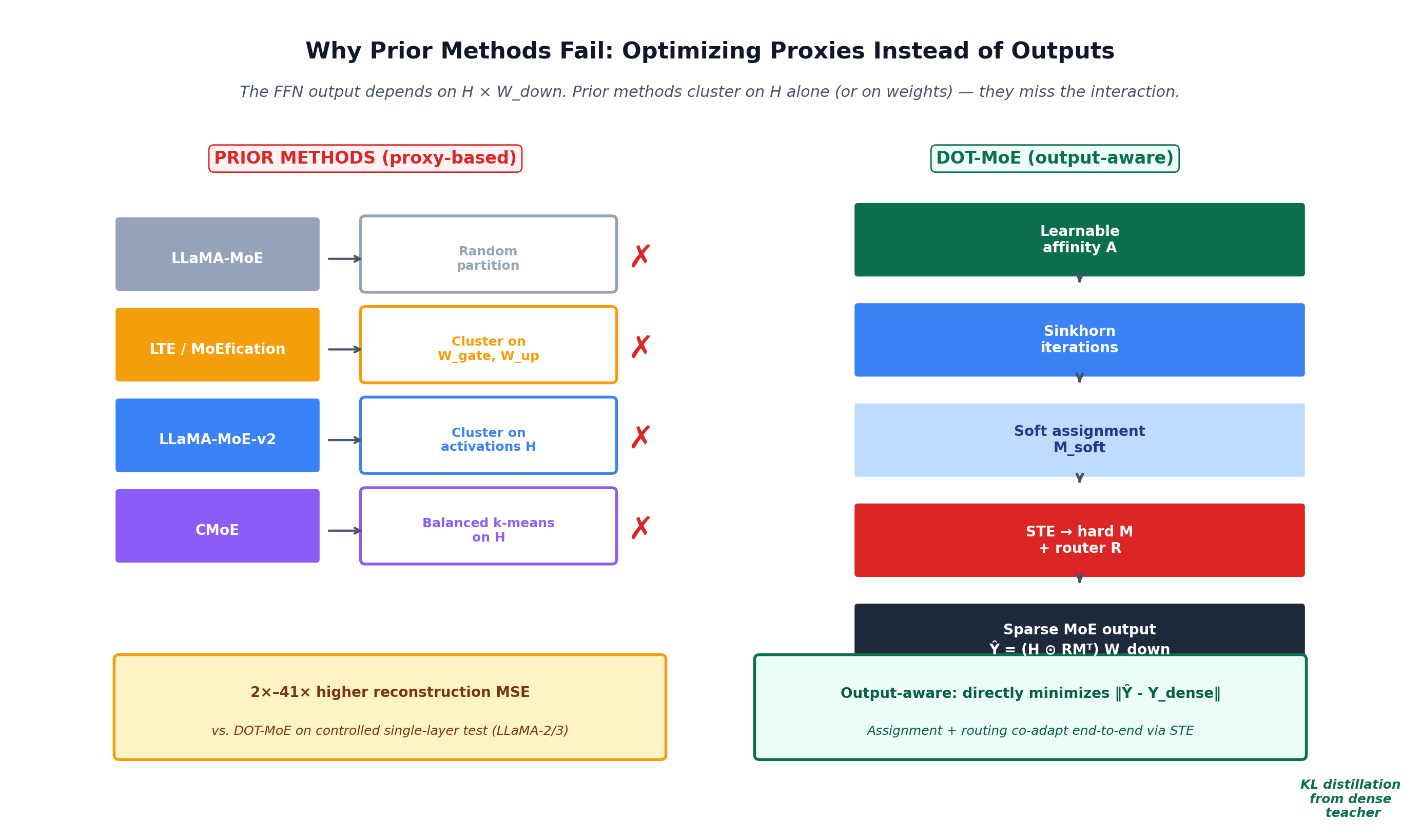
This is the central insight of the paper:
You cannot pick good experts by looking at inputs or activations. You must look at the output.
Everything else in DOT-MoE follows from this one observation.
Here is the reframing that makes everything click.
Reframe neuron-to-expert assignment as a transport problem:
d_ffn neurons is a unit of mass that must be shipped to exactly one expert.E experts is a bin with capacity exactly s (so s · E = d_ffn).i to expert e is a learnable score A[i,e].This is precisely the balanced optimal transport (OT) problem:

Where the transportation polytope is:

And the marginals are simply:

r = 1_{d_ffn} means each neuron ships exactly once. c = s·1_E means each expert receives exactly s neurons.
Three reasons, all from first principles:
Capacity is hard-coded as a constraint, not a soft penalty. Sinkhorn's marginal constraints guarantee every expert has exactly s neurons. No more "approximate balance" — balance is structural. Switch Transformer and LLaMA-MoE use auxiliary load-balancing losses that only encourage balance; DOT-MoE enforces it.
Assignment becomes jointly learnable with the router. The affinity matrix A is a parameter. Gradients from the reconstruction loss flow back into A, so the assignment adapts to the routing policy and vice versa. Prior methods freeze assignment first, then train a router on a fixed partition — they cannot co-adapt.
Output-aware by construction. The cost of an assignment is measured by how well the resulting sparse MoE reconstructs the dense FFN output — not by clustering on H or W_gate.
The optimum M* of the linear program above is a vertex of the transportation polytope — a {0,1} matrix. Two issues:
argmax over a polytope has no gradient, so A cannot be learned.d_ffn ~ 14k.Add an entropy term (Cuturi, 2013):

Where:

This strictly convexifies the problem, giving a unique interior solution with a beautiful closed form:

Where u ∈ ℝ_+^{d_ffn} and v ∈ ℝ_+^E are scaling vectors found by the Sinkhorn-Knopp algorithm: alternating row and column normalizations that converge linearly. As τ → 0, the solution approaches the discrete optimum; as τ → ∞, it approaches uniform.
The result is a soft, differentiable assignment M_soft ∈ [0,1]^{d_ffn × E}.
Here is the end-to-end DOT-MoE pipeline:

There are two coupled learnable components and one frozen component:
| Component | Shape | Status | Role |
|---|---|---|---|
Dense FFN weights W_gate, W_up, W_down |
d×d_ffn, d×d_ffn, d_ffn×d |
Frozen | The pre-trained dense model; provides teacher signal |
Affinity matrix A |
d_ffn × E |
Trained | Scores how well neuron i fits expert e |
Router weights W_r |
E × d |
Trained | Scores which experts each token should use |
Total trainable parameters: under 2% of the model.
For an input batch X ∈ ℝ^{n×d}:
Step 1 — Dense forward (frozen). Compute H = σ(X W_gate) ⊙ (X W_up) ∈ ℝ^{n×d_ffn} and the dense teacher logits z_dense.
Step 2 — Neuron-to-expert soft assignment (Sinkhorn). Compute K = A / τ, then run log-domain Sinkhorn iterations with marginals (1, s·1) to get M_soft.
Step 3 — Discretize via greedy rounding. Sort all d_ffn × E entries of M_soft in descending order. Walk down the list, assigning neuron i to expert e iff i is unassigned and e has capacity. Result: M ∈ {0,1}^{d_ffn × E}.
Step 4 — Token-to-expert routing. Compute router logits and probabilities:


Then pick top-k:
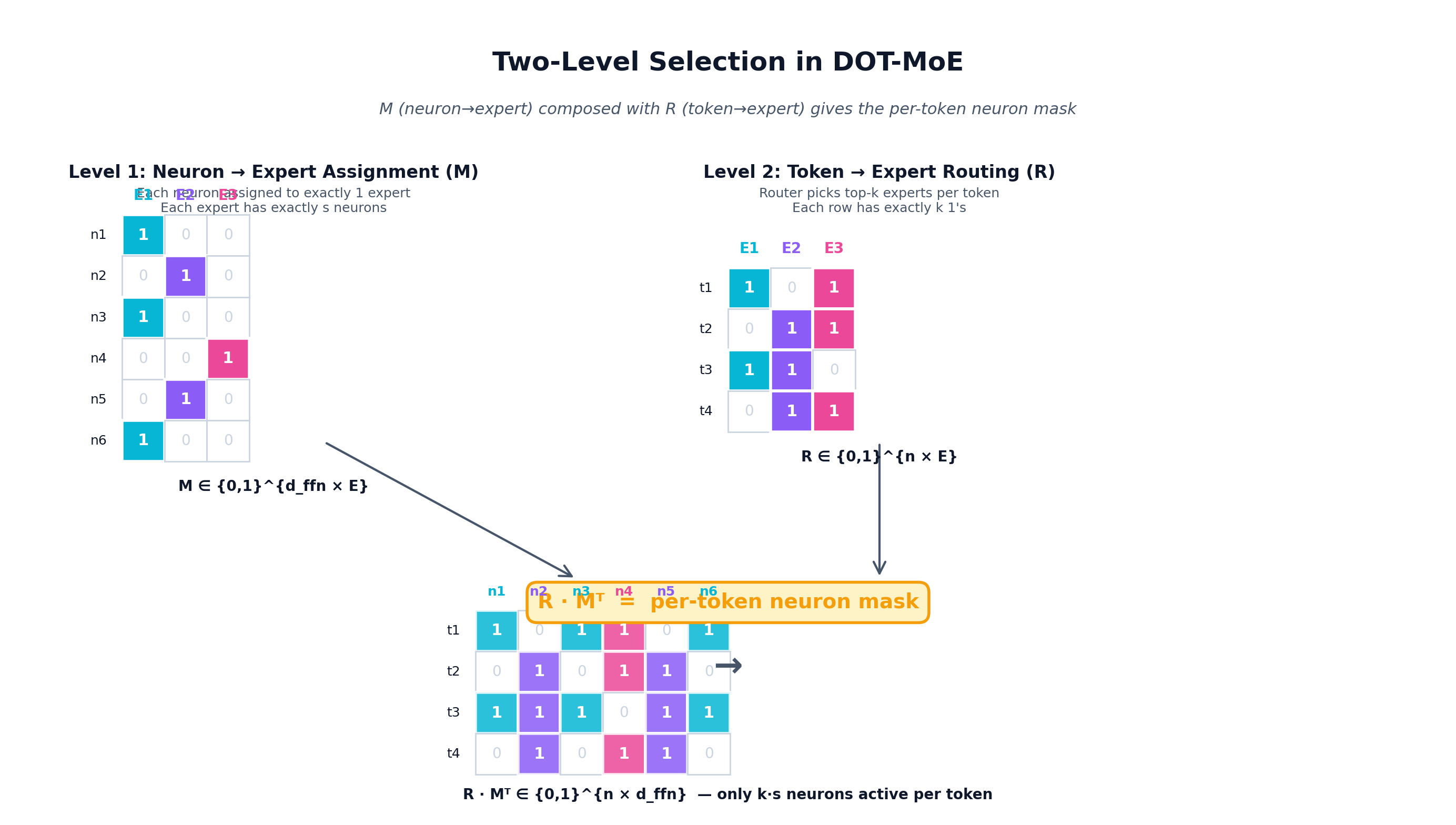
Step 5 — Sparse MoE forward (no separate expert weights materialized). Compose the two selections into a per-token neuron mask:

The matrix product R M^T ∈ {0,1}^{n×d_ffn} is the compositional mask: it answers "for token i, which neurons are alive?" by intersecting "which experts are active for i" (R) with "which neurons belong to each expert" (M). Each token activates exactly k · s neurons out of d_ffn.
Here is the two-level selection visualized:
Step 6 — Loss & backprop. Compute the total objective:

Where:
- L_KL = KL(z_dense || z_MoE) — distill the dense teacher's output distribution into the MoE student. This is the output-aware signal.
- L_CE — standard language modeling cross-entropy.
- L_z — router z-loss for stability:

L_bal — Switch-Transformer-style load balancing:
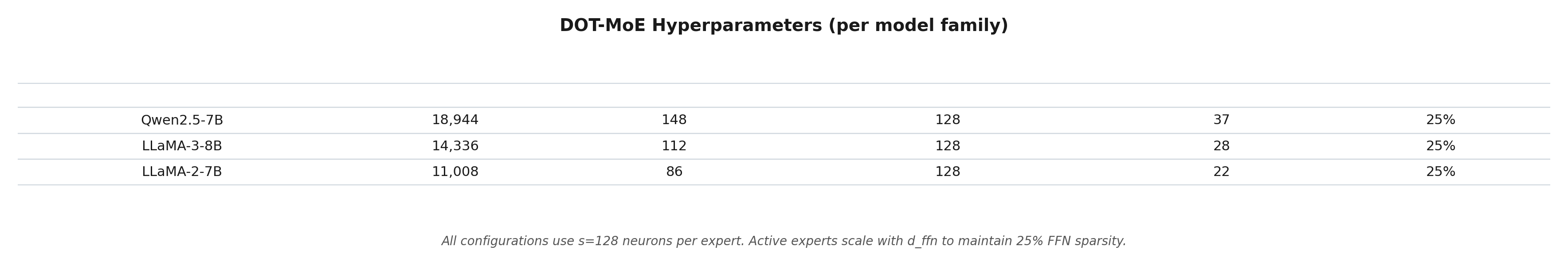
| Model | d_ffn |
E (experts) |
s (neurons/expert) |
k (active) |
Active % FFN |
|---|---|---|---|---|---|
| Qwen2.5-7B | 18,944 | 148 | 128 | 37 | 25% |
| LLaMA-3-8B | 14,336 | 112 | 128 | 28 | 25% |
| LLaMA-2-7B | 11,008 | 86 | 128 | 22 | 25% |
Other key settings:
- Temperature annealed linearly τ: 1.0 → 0.1 during warmup (high τ = explore, low τ = commit).
- A kept in FP32 regardless of model dtype (Sinkhorn is sensitive to precision).
- Log-domain Sinkhorn (avoids underflow when τ is small).
- Optimizer: AdamW + cosine LR + linear warmup.
- Hardware: 8× H100. Alignment: 3,500 steps, <3 hours for LLaMA-3-8B.
- Training data: Dolmino-mix. 1.2B tokens for downstream fine-tuning.
Once training converges:
M.e, slice rows of W_gate, W_up and columns of W_down corresponding to neurons C_e = {i : M[i,e]=1}.E real, independent FFN experts — a standard MoE architecture compatible with vLLM, FasterTransformer, etc.At inference time there is no Sinkhorn, no STE, no alignment overhead. It is just a vanilla sparse MoE.
The same formulation extends to multi-head attention: treat heads as the units to be grouped. For Qwen2.5-7B: N_h=28 heads → E_attn=14 head-experts of s_h=2 heads each, k_attn=7 active. Affinity matrix A_attn ∈ ℝ^{N_h × E_attn} is trained identically. For GQA, assignment operates on query heads; KV heads are always computed; sparsity lives in Q and O projections.
We will see the attention results in Section 10.
Sinkhorn is the workhorse that makes DOT-MoE tractable. Let's look at exactly what it does.
The Sinkhorn-Knopp algorithm performs alternating row and column normalizations that converge linearly to the unique solution satisfying the marginal constraints.
Here is the algorithm (in log-domain for numerical stability):
Algorithm 1: Log-Domain Sinkhorn for Balanced Assignment
─────────────────────────────────────────────────────────
Input : A ∈ ℝ^{d_ffn × E}, temperature τ, iterations N
Output: M_soft ∈ [0,1]^{d_ffn × E}

1. K ← A / τ
2. u ← 0,  v ← log(s) · 1_E
3. for t = 1 to N:
4.     u ← -logsumexp(K + v, dim=1)              # row normalize (each neuron → sum 1)
5.     v ← log(s·1_E) - logsumexp(K + u, dim=0)  # col normalize (each expert → sum s)
6. M_soft ← exp(K + u + v)
Here is the algorithm visualized across iterations:
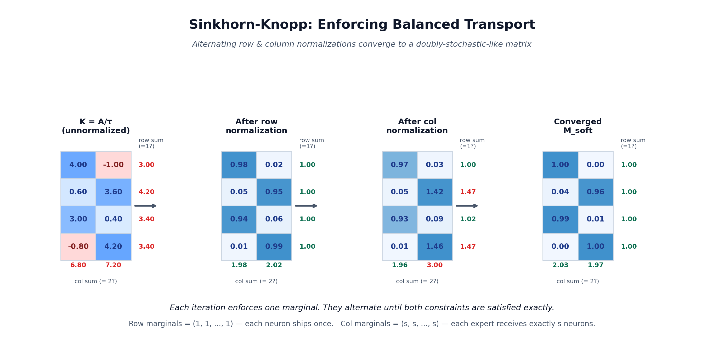
Each iteration enforces one marginal. They alternate until both constraints are satisfied exactly. After ~10 iterations, M_soft converges to a soft assignment that:
s (each expert has exactly s neurons' worth of mass).The greedy rounding then converts this to a hard {0,1} assignment. Because Sinkhorn already accounts for capacity globally (redistributing mass when experts are over-demanded), the gap between soft and hard assignments is small.
When τ is small (e.g., 0.1), exp(A/τ) overflows easily. The log-domain formulation operates entirely in log-space, using logsumexp instead of explicit exponentiation. This makes Sinkhorn numerically stable even with thousands of neurons and experts.
Both M (from greedy rounding) and R (from top-k) are non-differentiable. If you cannot differentiate through them, you cannot train A or W_r end-to-end.
The solution: Straight-Through Estimator (STE) (Bengio et al., 2013).
The STE uses the hard decisions in the forward pass but routes gradients through the soft counterparts in the backward pass:


Where sg(·) is the stop-gradient operator. In the forward pass you use the discrete decisions (so the model genuinely is sparse). In the backward pass you pretend the soft versions were used, so gradients flow into A (through M_soft) and into W_r (through P).
Here is the STE concept visually:
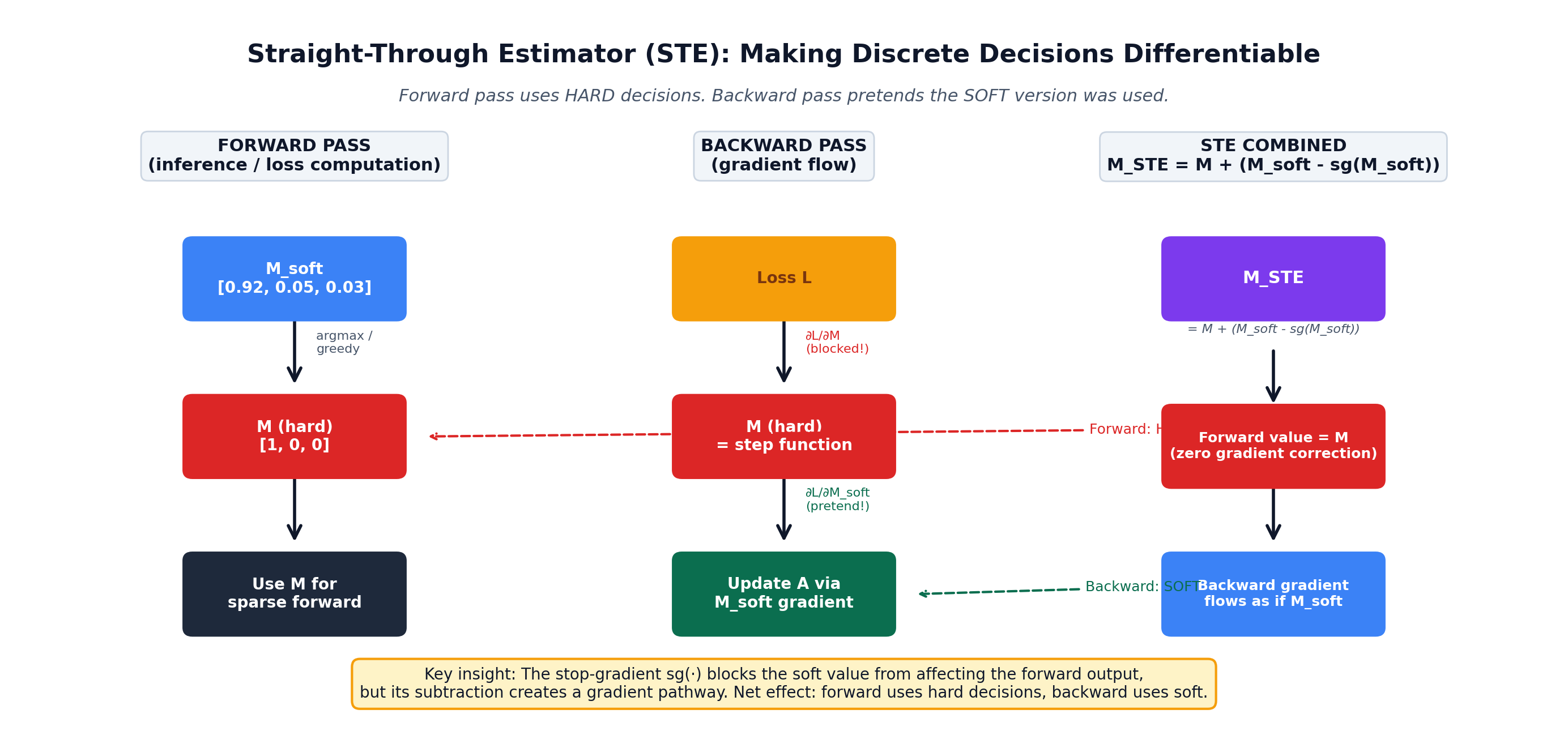
The stop-gradient sg(·) blocks the soft value from affecting the forward output, but its subtraction creates a gradient pathway. Net effect: forward uses hard decisions, backward uses soft.
This is the key that lets assignment and routing co-adapt end-to-end. Prior methods cannot do this — they freeze M first, then train W_r. They cannot recover from a bad initial partition.
This is the heart of why DOT-MoE works. Let's trace exactly what happens during training.
Consider what happens to a single affinity entry A[i,e] (the score for putting neuron i in expert e).
Forward: A[i,e] enters M_soft[i,e], which (after rounding) determines whether neuron i is in expert e. If yes, and if expert e is activated for token t (router decision R[t,e]=1), then neuron i contributes H[t,i] · W_down[i,:] to the MoE output for token t.
Loss: L_KL compares the MoE output Y_hat against the dense teacher output. If neuron i's contribution via expert e helped reconstruct the teacher output for the tokens routed to e, then L_KL is lower with this assignment than without it.
Backward (STE): The gradient ∂L/∂A[i,e] is computed as if M_soft were used. A positive gradient says "this assignment hurt reconstruction — make it less likely." A negative gradient says "this assignment helped — make it more likely."
Update: A[i,e] moves to increase the affinity for assignments that maximally preserve the dense output.
The affinity A and the router W_r are mutually informative. Here is the loop:
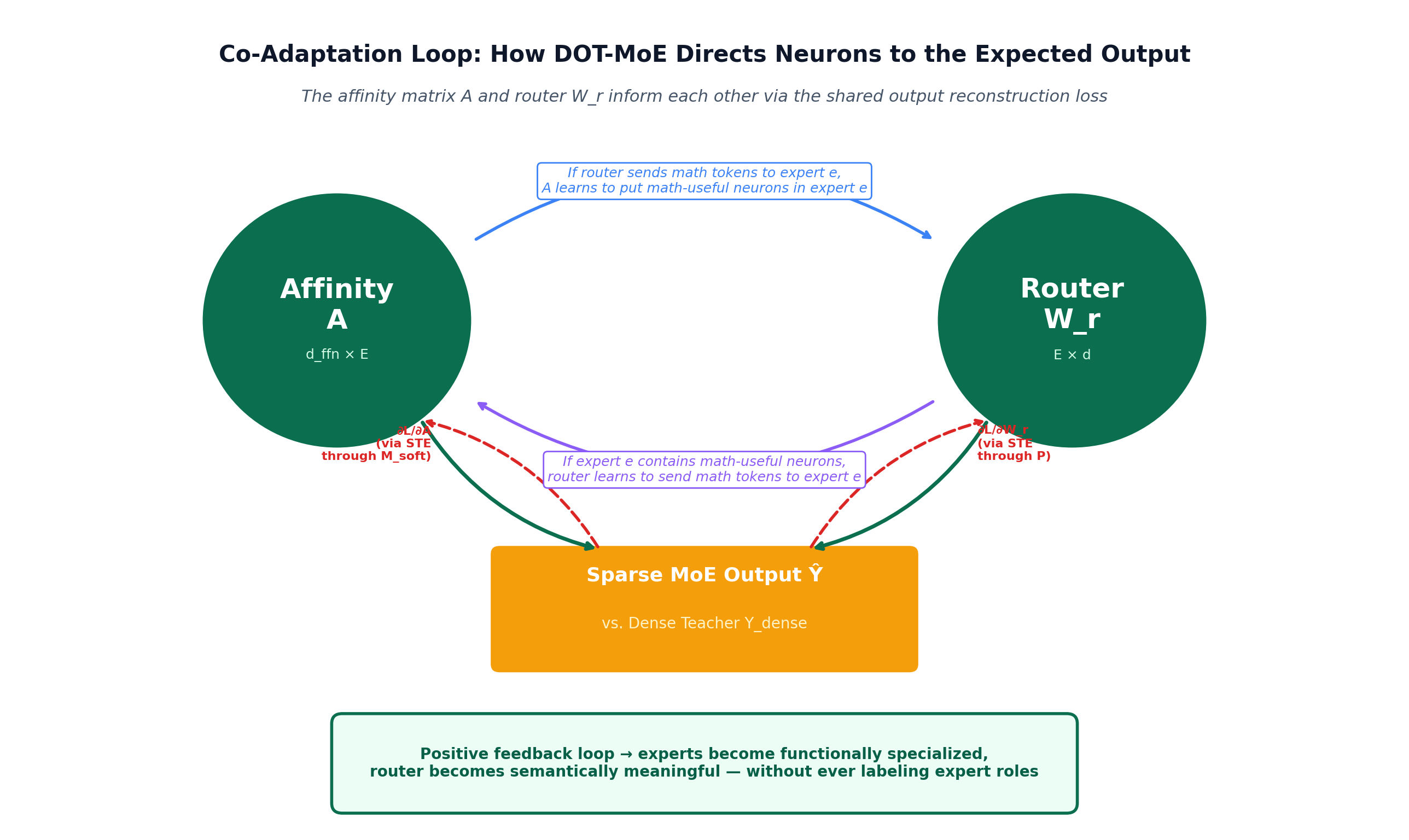
This positive feedback loop is exactly what heuristic methods cannot achieve because they decouple the two stages. The router and the expert structure co-adapt — without ever being told what "math" is or which expert should handle it.
The capacity constraint (M^T 1 = s·1_E) is non-negotiable — enforced by Sinkhorn's column normalization. This guarantees:
E equally-sized experts to choose from.Switch Transformer and Shazeer-style MoEs use soft load-balancing losses (a penalty term in the loss). These can be violated; they cannot guarantee exact balance. DOT-MoE bakes balance into the feasible set of the optimization.
To make this concrete, let's do a tiny dry run. Suppose:
d_ffn = 6 neurons, E = 2 experts, s = 3 neurons per expert, k = 1 active expert per token.x, with intermediate activation H = [0.9, 0.1, 0.5, 0.8, 0.2, 0.7] and W_down columns that produce dense output y_dense = H · W_down = [1.0] (scalar for simplicity).ASay after a few training steps:
A = [[ 2.0, -0.5],     ← neuron 0 prefers expert 0
     [ 0.3,  1.8],     ← neuron 1 prefers expert 1
     [ 1.5,  0.2],     ← neuron 2 prefers expert 0
     [-0.4,  2.1],     ← neuron 3 prefers expert 1
     [ 1.9,  0.1],     ← neuron 4 prefers expert 0
     [ 0.5,  1.7]]     ← neuron 5 prefers expert 1
K = [[ 4.0, -1.0],
     [ 0.6,  3.6],
     [ 3.0,  0.4],
     [-0.8,  4.2],
     [ 3.8,  0.2],
     [ 1.0,  3.4]]
Marginals: r = [1,1,1,1,1,1] (each neuron ships once), c = [3,3] (each expert receives 3).
Iteration 1 — row normalize (each row should sum to 1):
After softmax over rows, M1 looks approximately like:
M1 ≈ [[1.00, 0.00],
      [0.05, 0.95],
      [0.99, 0.01],
      [0.00, 1.00],
      [1.00, 0.00],
      [0.08, 0.92]]

column sums = [3.13, 2.87]   ← not yet [3, 3]
Iteration 2 — col normalize (each col should sum to 3), then renormalize rows, and so on. After ~10 iterations:
M_soft ≈ [[1.00, 0.00],
          [0.04, 0.96],
          [0.99, 0.01],
          [0.00, 1.00],
          [1.00, 0.00],
          [0.06, 0.94]]

column sums ≈ [3.09, 2.91]   ← approaching [3, 3]
Sort all entries descending. Pick (0,0)=1.00, (4,0)=1.00, (2,0)=0.99 → expert 0 now full (capacity 3). Pick (3,1)=1.00, (1,1)=0.96, (5,1)=0.94 → expert 1 full.
M = [[1, 0],
     [0, 1],
     [1, 0],
     [0, 1],
     [1, 0],
     [0, 1]]

Expert 0 = {neurons 0, 2, 4}
Expert 1 = {neurons 1, 3, 5}
Router logits L = x · W_r^T = [0.7, -0.3] → P = softmax(L) = [0.73, 0.27] → top-1 = expert 0.
R = [[1, 0]]
R · M^T = [[1, 0]] · [[1, 1, 1, 0, 0, 0],
                     [0, 0, 0, 1, 1, 1]] = [[1, 1, 1, 0, 0, 0]]

H ⊙ (R · M^T) = [0.9, 0.1, 0.5, 0, 0, 0]
Y_hat = 0.9 · W_down[0] + 0.1 · W_down[1] + 0.5 · W_down[2]
Suppose Y_hat = 0.7 but y_dense = 1.0. Loss L = (0.7 - 1.0)^2 = 0.09.
Backward via STE (gradient flows as if M_soft were used):
H[3]=0.8 is large and W_down[3] would have helped), then A[3,0] gets a negative gradient (increase affinity), and A[3,1] gets a positive gradient (decrease affinity).A[3,0] rises, A[3,1] falls. Next iteration, Sinkhorn may move neuron 3 to expert 0 (subject to capacity — some other neuron must move out).If many "high-H" tokens like this one prefer expert 0, the router's W_r[0] strengthens, and the affinity matrix reorganizes so expert 0 ends up with the neurons most useful for high-H tokens.
This is the "directing neurons to the expected output" loop in action.
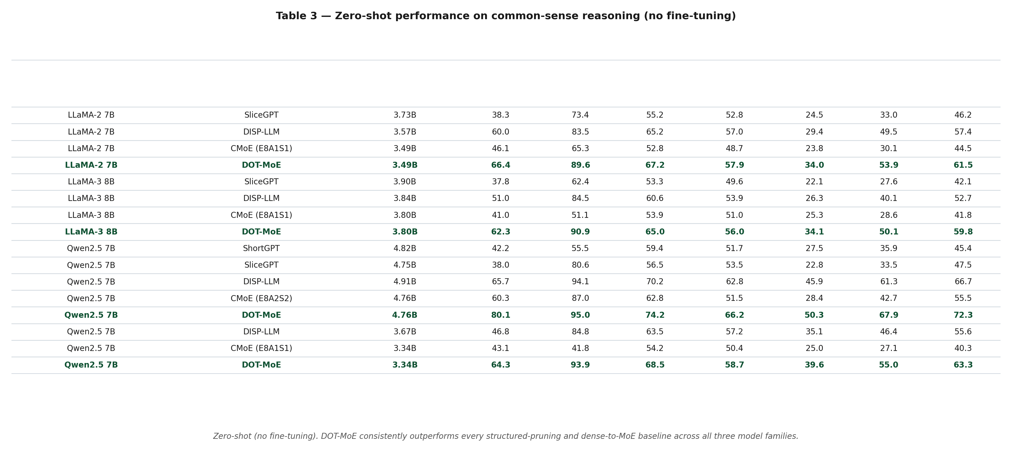
The authors evaluate on three model families — LLaMA-2-7B, LLaMA-3-8B, Qwen2.5-7B — across six common-sense reasoning benchmarks (BoolQ, SciQ, PIQA, Winogrande, ARC-Challenge, HellaSwag), using lm-evaluation-harness.
First, the headline number on LLaMA-2-7B at 50% parametric budget:
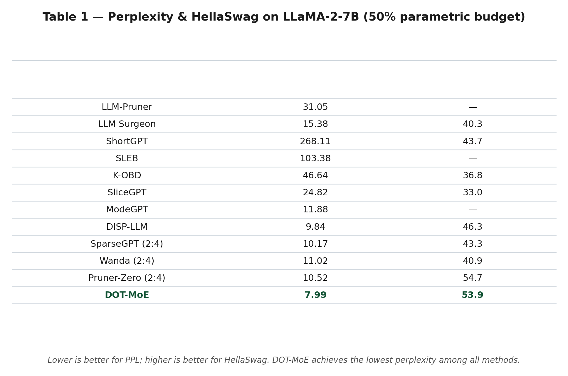
DOT-MoE achieves the lowest perplexity (7.99) among all methods — beating the SOTA structured-pruning method DISP-LLM (9.84) by a substantial margin, and competitive with semi-structured pruning methods (which have more freedom to hit any target sparsity).
This is where DOT-MoE really shines. Without any fine-tuning at all — just alignment:
The bar chart makes the gap clearer:
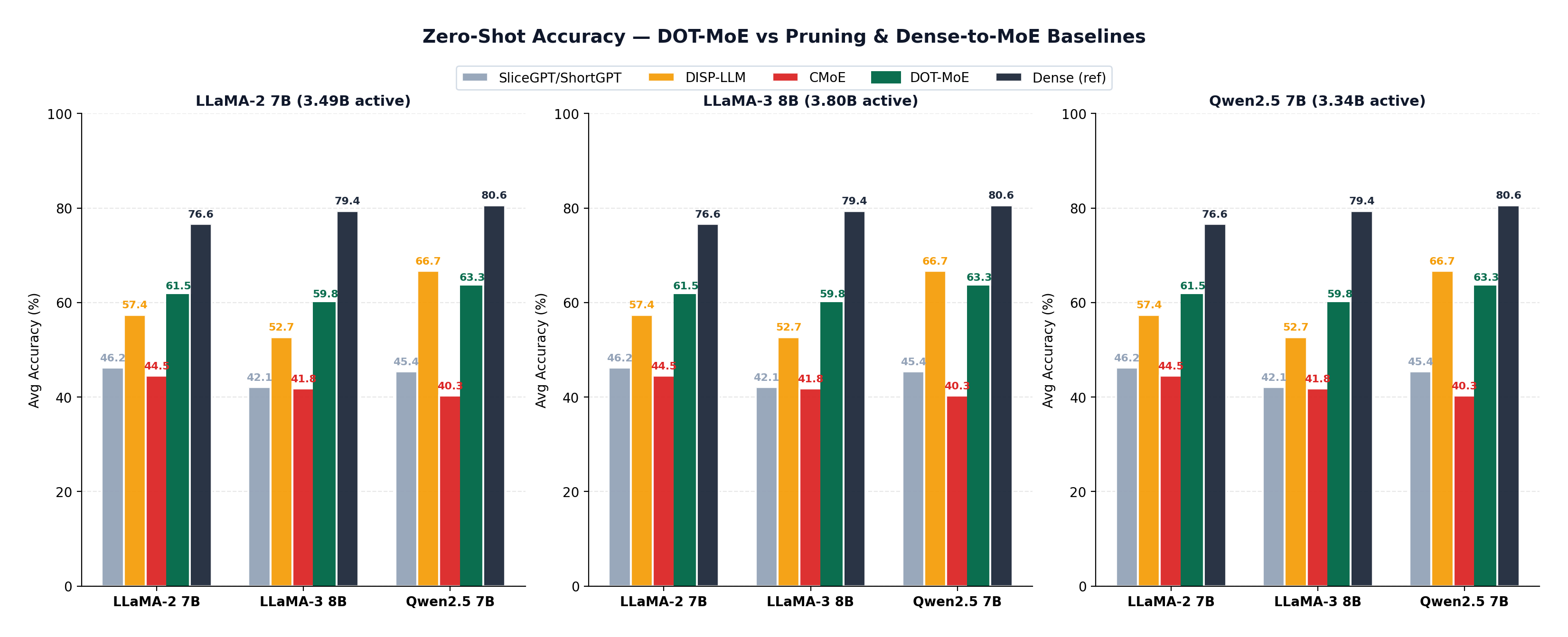
On LLaMA-3-8B, DOT-MoE achieves 59.8% average accuracy zero-shot, vs. CMoE at 41.8% — an 18-point gap with zero additional training.
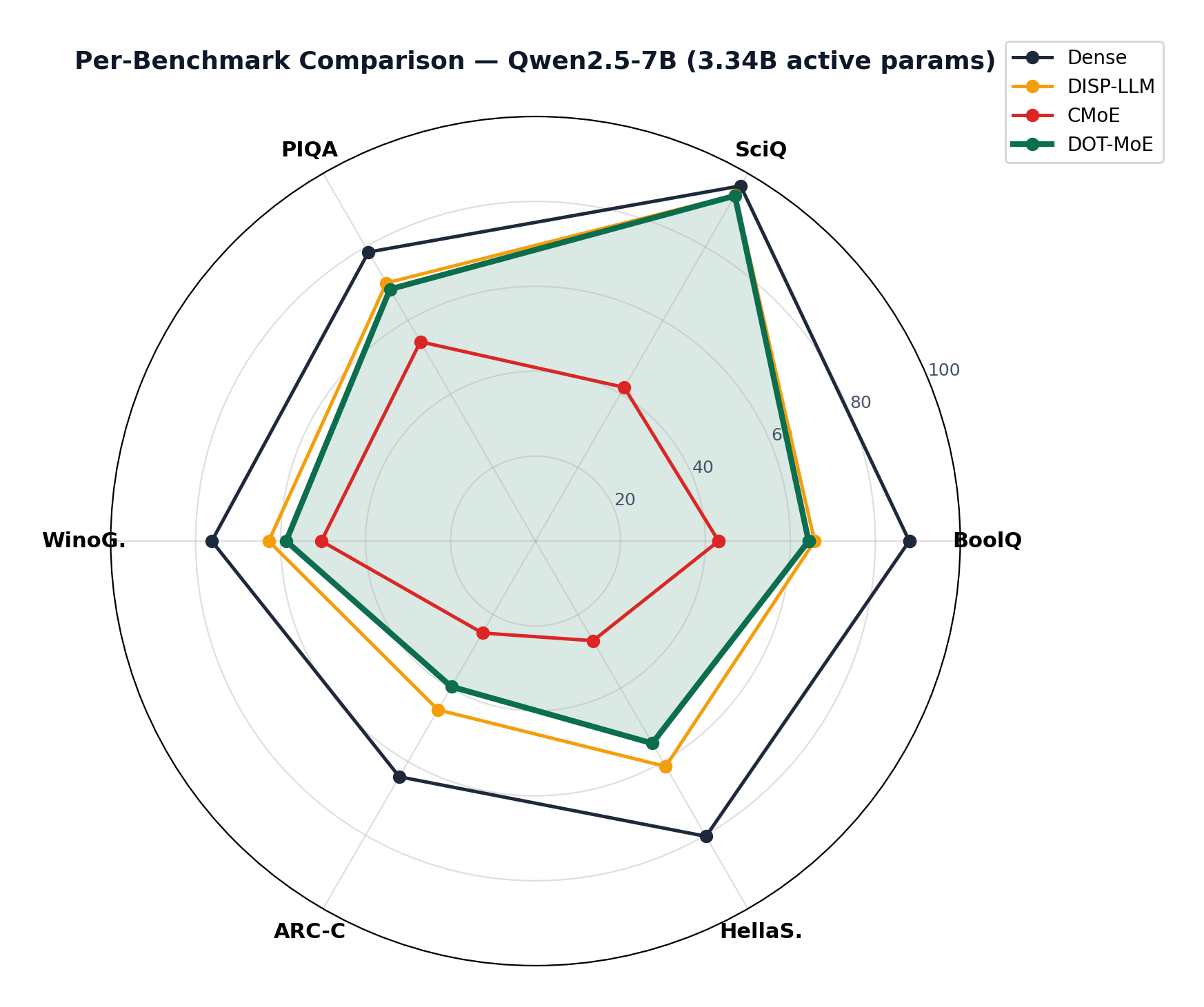
The radar chart shows per-benchmark detail for Qwen2.5-7B:
After 1.2B tokens of fine-tuning on Dolmino-mix:
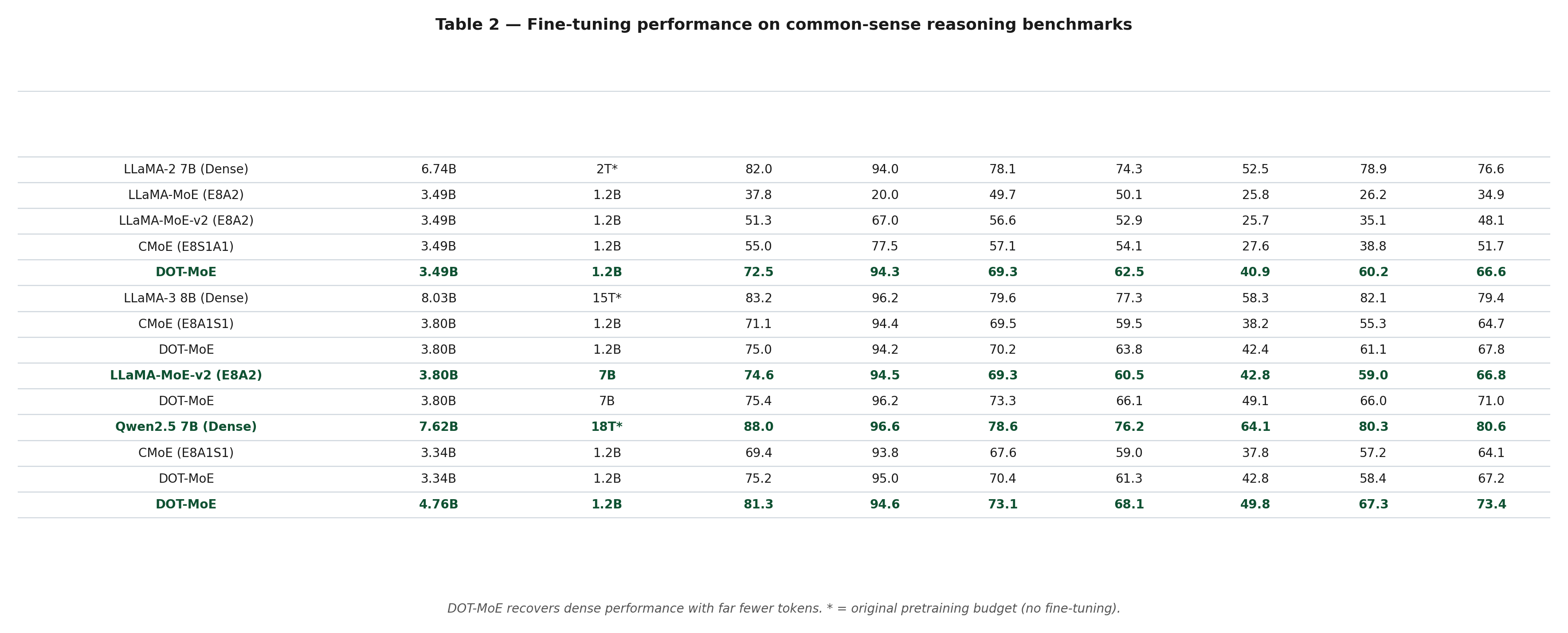
DOT-MoE closes the gap to the dense model rapidly. On Qwen2.5-7B with 1.2B FT tokens, DOT-MoE achieves 73.4% average accuracy vs. the dense model's 80.6% — recovering most of the gap with 50% active parameters.
The headline claim: "Retains 90% of dense performance at 50% parametric count."
LTE (Zheng et al., 2024) uses sigmoid threshold routing, which activates a variable number of experts per token — unpredictable compute, incompatible with standard fused-MoE kernels. DOT-MoE uses softmax top-k for fixed per-token compute:
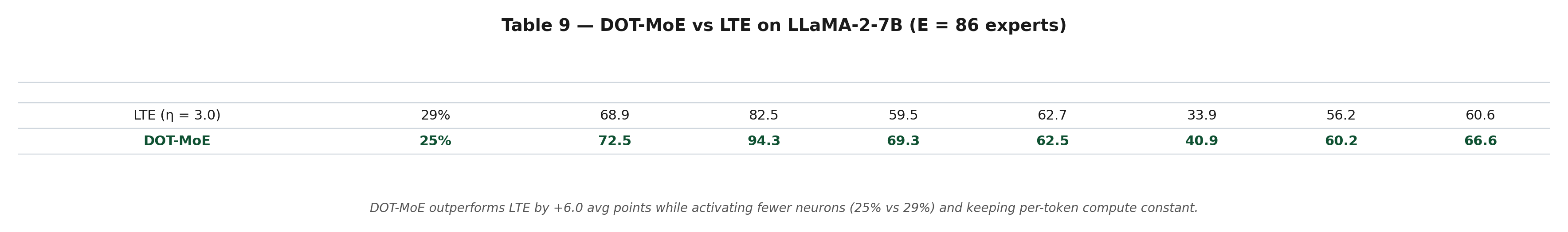
DOT-MoE beats LTE by +6.0 points while activating fewer neurons (25% vs 29%).
The same formulation extends to attention heads:
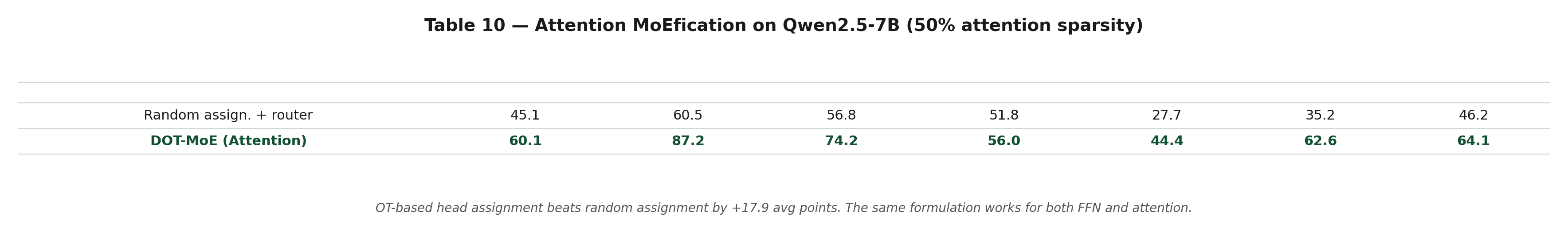
On Qwen2.5-7B at 50% attention sparsity, DOT-MoE beats random head-assignment by +17.9 points. The OT formulation works for both FFN and attention.
DOT-MoE gets better at scale:
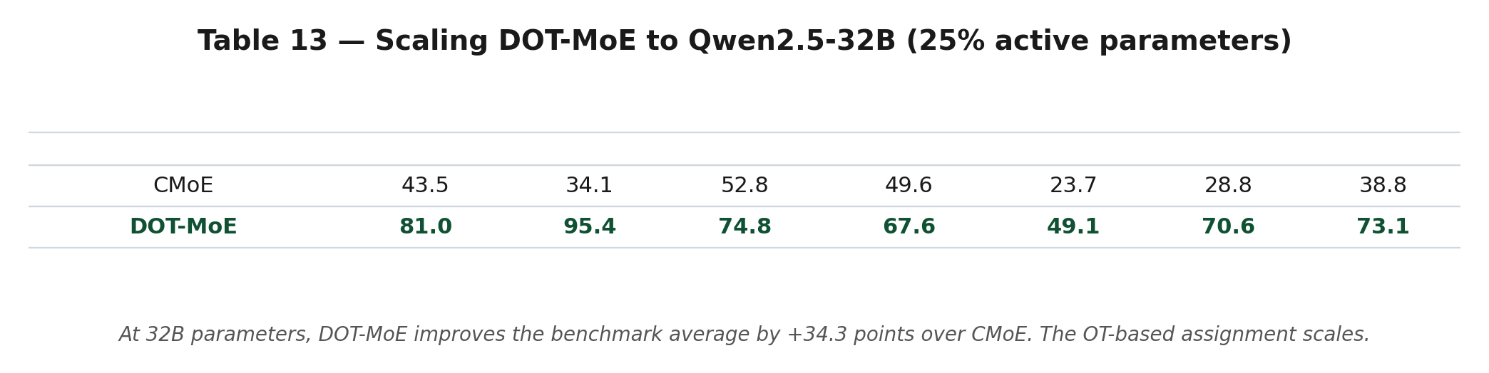
On Qwen2.5-32B at 25% active params, DOT-MoE improves over CMoE by +34.3 points (73.1 vs 38.8). The OT-based assignment holds up as model scale increases.
Per-token routing is length-agnostic:
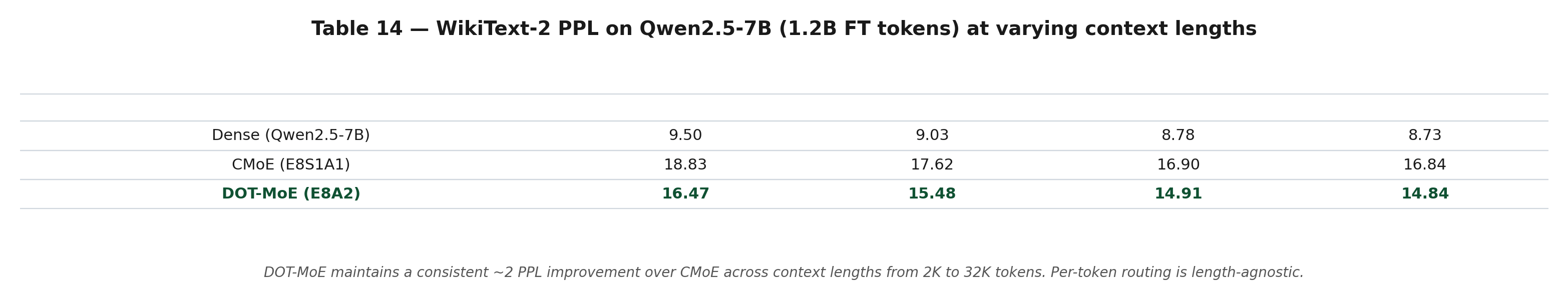
DOT-MoE maintains a consistent ~2 PPL improvement over CMoE across context lengths from 2K to 32K tokens.
The paper's ablation studies reveal four insights worth understanding deeply.
From the paper's Figure 1(a):
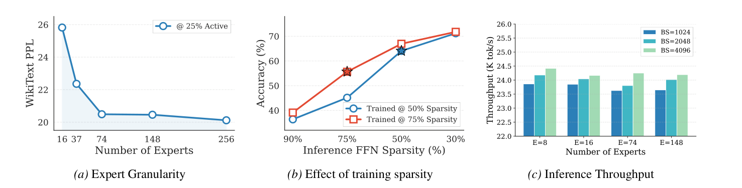
Increasing the number of experts (E ∈ {16, 37, 74, 148, 256}) improves performance up to a point, then saturates. Critically, this differs from prior methods — CMoE and LLaMA-MoE-v2 actually degrade when E goes from 8 to 16 due to routing complexity. The authors tried CMoE with E=37, top-k=9 and got >5K WikiText PPL — the model completely collapsed.
Observation 1: Routing benefits from fine-grained experts up to a point, beyond which additional experts provide limited returns.
A natural concern: does increasing E slow down inference? The answer is no, thanks to vLLM's fused MoE kernels. All expert FFNs are concatenated as W_fused = [W_1, ..., W_E] along the expert dimension, and a single large GEMM is executed regardless of E. Since the total fused intermediate dimension (E × s) and active neurons per token (k × s) remain constant, GEMM sizes — and thus throughput — are largely unaffected.
Observation 2: Fine-grained experts incur no throughput penalty with fused MoE kernels when active parameters are held constant.
This one is counterintuitive. The authors trained two Qwen2.5-7B models: one at 50% FFN sparsity, one at 75%. Then they evaluated both across a range of inference sparsities:
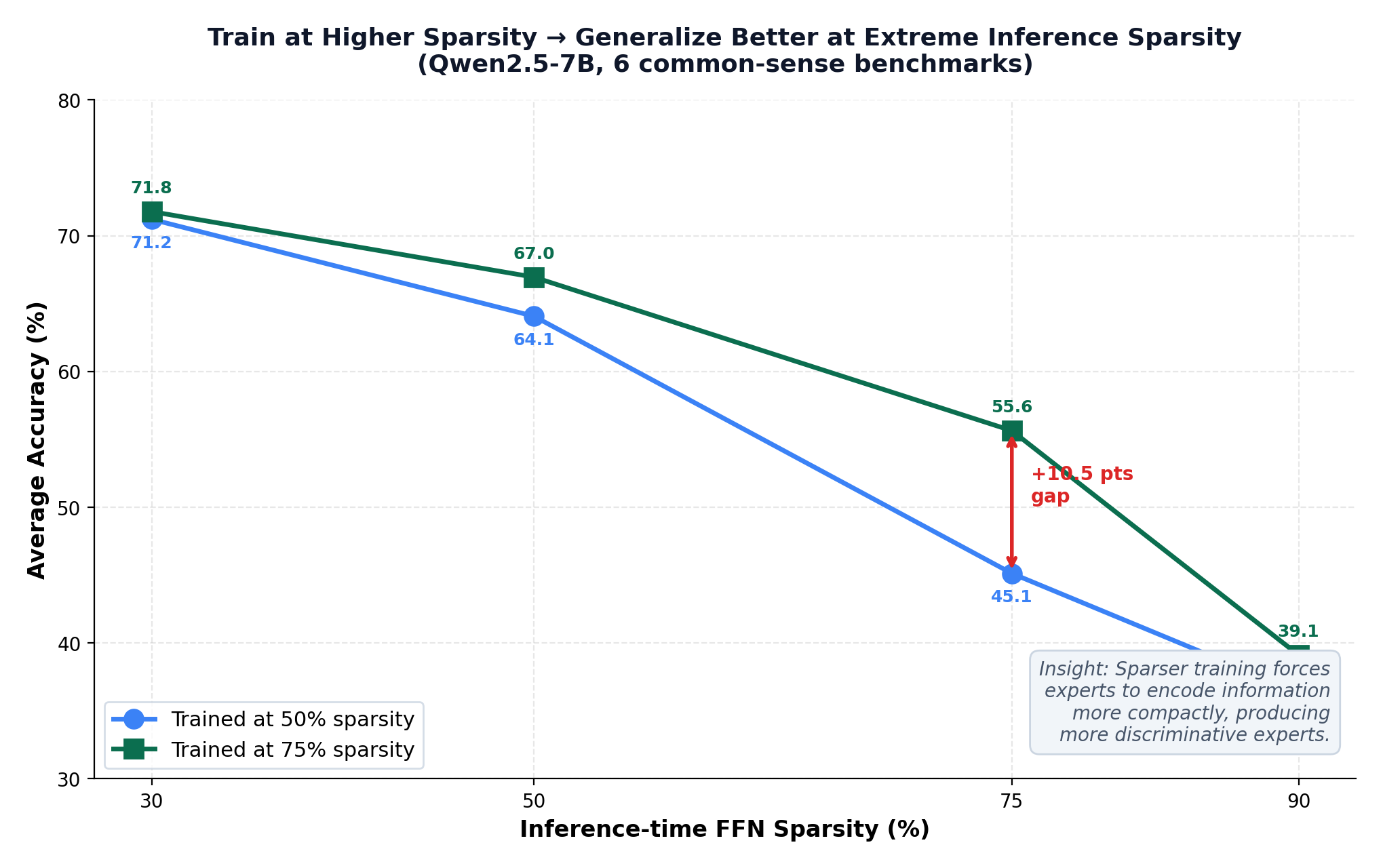
The model trained at 75% sparsity outperforms the 50%-trained model across the board — even when both are evaluated at 50% inference sparsity. At 75% inference sparsity, the gap is +10.5 points.
The explanation: when you train with fewer active experts, the model learns to encode information more efficiently within each expert, producing more compact and discriminative representations. The experts become better, not just sparser.
Observation 3: Training at higher sparsity yields experts that generalize better across varying inference sparsities.
From the paper's Figure 2:
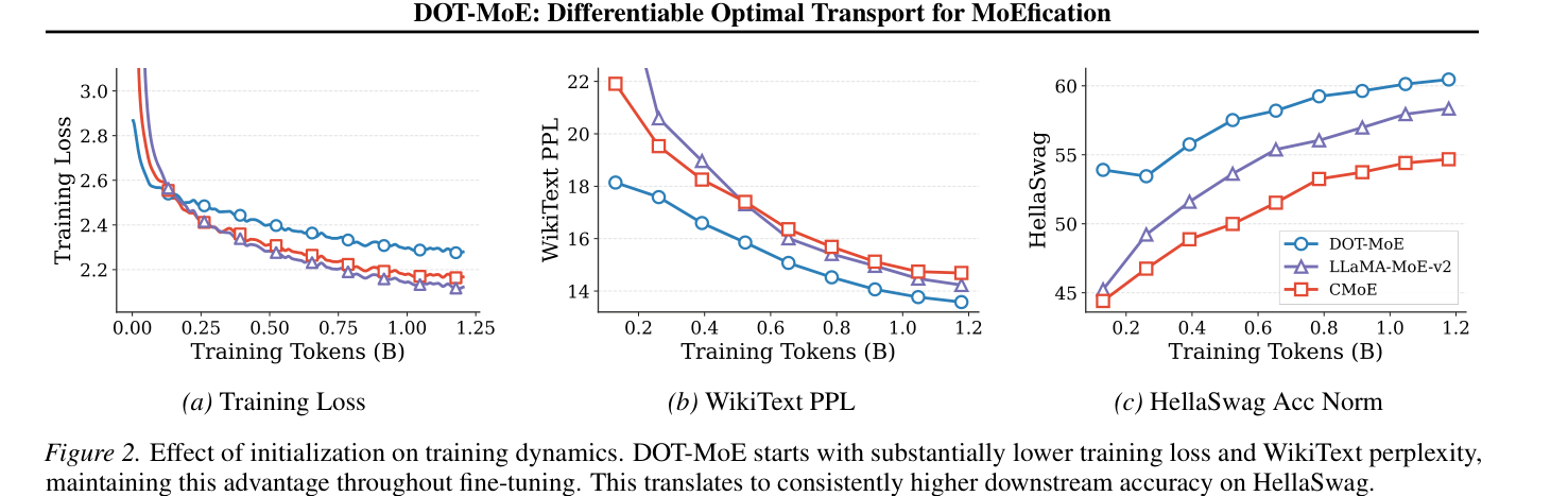
DOT-MoE starts with substantially lower training loss compared to CMoE and LLaMA-MoE-v2. While all methods reduce training loss over time, CMoE and LLaMA-MoE-v2 exhibit classic overfitting symptoms — training loss drops but validation PPL rises, downstream accuracy degrades.
DOT-MoE continues to improve on both validation perplexity and downstream task performance throughout training.
Observation 4: Output-aware initialization achieves superior training generalization, whereas heuristic methods exhibit overfitting.
A skeptic might say: "DOT-MoE wins because it uses more experts." The authors control for this by running DOT-MoE at CMoE's own setting (E=8, top-k=2):
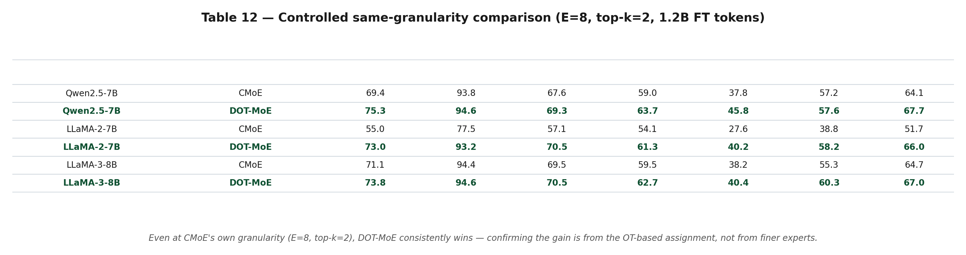
Even at CMoE's own granularity, DOT-MoE wins across all three architectures. The gain comes from the OT-based assignment, not from finer experts.
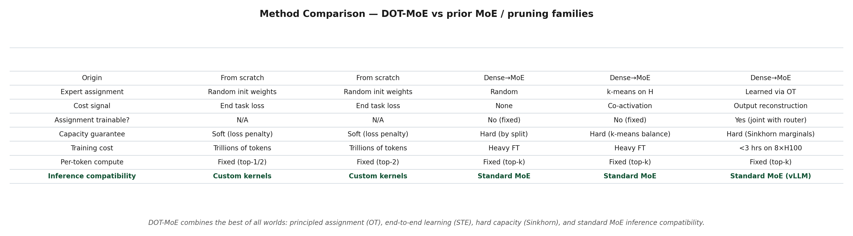
Let's put DOT-MoE in context. Here is a structural comparison of dense-to-MoE methods:
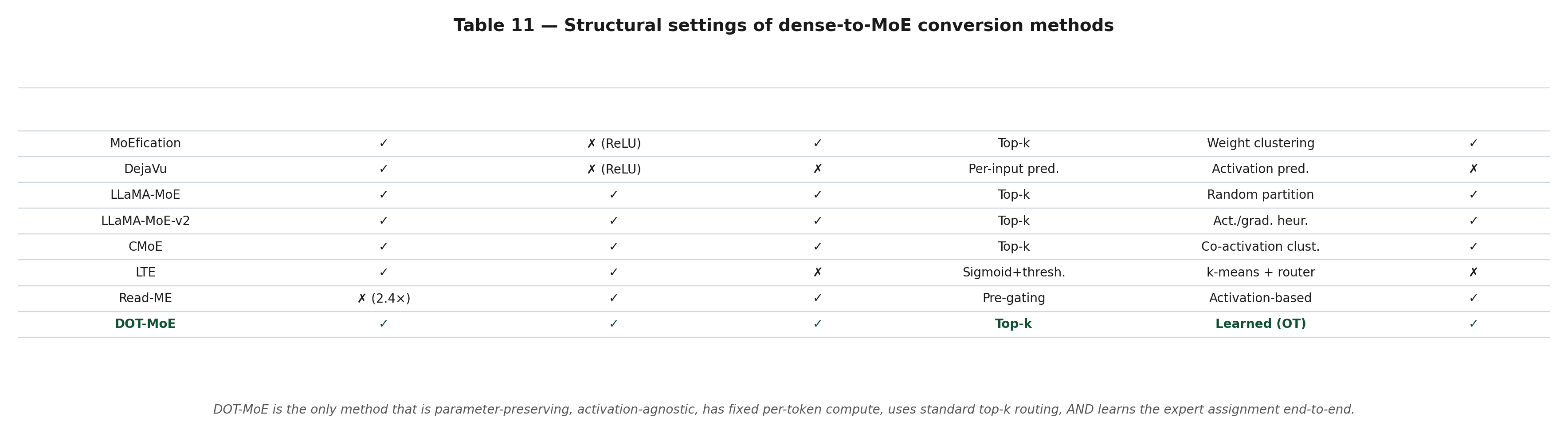
DOT-MoE is the only method that is:
- Parameter-preserving (✓)
- Activation-agnostic (✓ — works for any activation, not just ReLU)
- Fixed per-token compute (✓)
- Standard top-k routing (✓ — compatible with vLLM)
- Learned expert assignment (✓ — all others use heuristics)
- Serves as a standard MoE (✓)
| Aspect | Switch Transformer | DOT-MoE |
|---|---|---|
| Origin | Trained from scratch | Converted from dense |
| Routing | top-1 softmax | top-k softmax |
| Assignment | Pre-defined random init | Learned via OT |
| Load balance | Soft auxiliary loss | Hard marginal constraint |
| Training cost | Trillions of tokens from scratch | 1.2B tokens + alignment |
Switch must learn the entire model from scratch, including every expert's weights. DOT-MoE reuses dense weights and only learns the partition + router. Per-token inference cost is comparable, but training cost is orders of magnitude lower.
Same family — trained from scratch with top-2 routing, random-init independent expert networks, soft load-balancing. Same problem: you pay the pretraining tax again.
DOT-MoE's experts are not random networks — they are principled groupings of pre-trained neurons that provably reconstruct the dense output. You get MoE-like inference speedup without re-pretraining.
| Aspect | LLaMA-MoE | LLaMA-MoE-v2 | CMoE | DOT-MoE |
|---|---|---|---|---|
| Assignment | Random | Act + grad importance | Balanced k-means on H | Learned via OT |
| Cost signal | None | Activation magnitude | Co-activation in H | Output reconstruction |
| Assignment trainable? | No (fixed) | No (fixed) | No (fixed) | Yes |
| Joint with router? | No (two-stage) | No (two-stage) | No (two-stage) | Yes (end-to-end) |
| Capacity guarantee | Yes (by construction) | Yes | Yes (k-means balance) | Yes (Sinkhorn marginals) |
| Needs heavy FT? | Yes | Yes | Yes | Minimal |
Prior methods fix a sub-optimal partition (chosen by a proxy) and then must recover via fine-tuning. DOT-MoE starts with a near-optimal partition (output-aware) and co-adapts it with the router.
Pruning permanently deletes parameters. MoEfication keeps all parameters but activates a subset per token. The paper's framing is sharp: MoEfication is "dynamic structural pruning conditioned on input."
Empirically on LLaMA-2-7B at 50% params: SliceGPT PPL=24.82, DISP-LLM PPL=9.84, SparseGPT PPL=10.17, DOT-MoE PPL=7.99. Even against semi-structured pruning (which has more freedom to hit any target sparsity), DOT-MoE wins.
A dense LLM trained from scratch with the same compute budget as DOT-MoE (alignment + 1.2B FT tokens) would be much smaller and much worse. DOT-MoE lets you take an already-pretrained dense model and produce a sparse MoE that:
Here is the side-by-side comparison:
DOT-MoE combines the best of all worlds: principled assignment (OT), end-to-end learning (STE), hard capacity (Sinkhorn), and standard MoE inference compatibility.
Prior MoE papers ask: "How do we train a sparse model from scratch?"
DOT-MoE asks: "Given that we already have a great dense model, what is the optimal way to extract a sparse MoE from it?"
This reframing matters because the industry has converged on a small number of extremely expensive dense foundation models. Retraining them as MoEs from scratch is wasteful and unstable. DOT-MoE shows you can get MoE-like inference efficiency without paying the pretraining tax again — and you can do it in 3 hours on 8 GPUs.
Profiled on 8× H100 (from Appendix H):
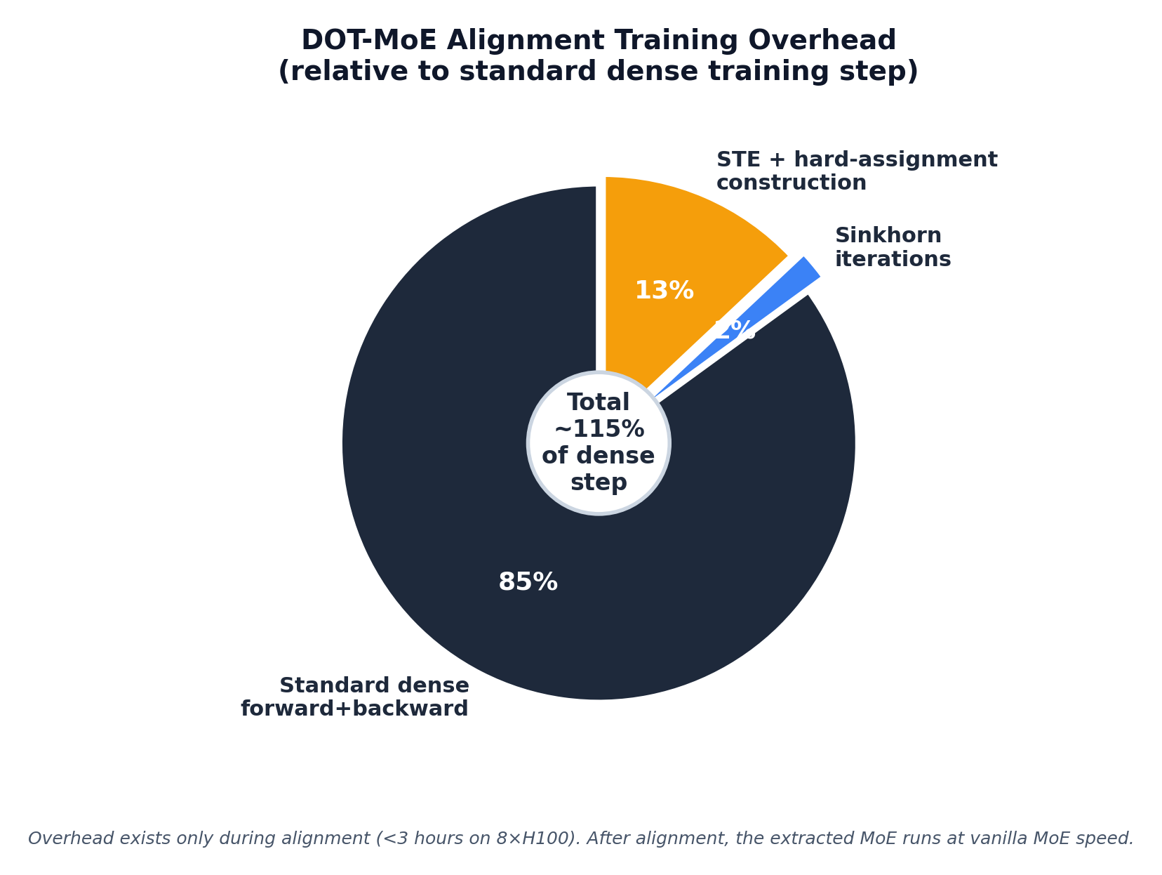
After alignment, the model is a standard MoE. With vLLM fused kernels:
W_fused = [W_1, ..., W_E] along the expert dimension.k · s neurons are active.(batch, k·s) × (k·s, d), regardless of E.So you can crank up expert granularity (more, smaller experts → finer routing) for free in inference. Prior methods (CMoE, LLaMA-MoE-v2) actually degrade when E goes from 8 → 16.
A (d_ffn × E) and W_r (E × d) are trained — <2% of model params. The dense weights are frozen, so no optimizer state for them.The paper is honest about gaps:
A. A data-driven initialization (weight correlations, precomputed activation statistics) could accelerate Sinkhorn convergence. Future work.To verify that experts actually specialize, the authors visualize expert output activations via t-SNE for layer 9 of Qwen2.5-7B:
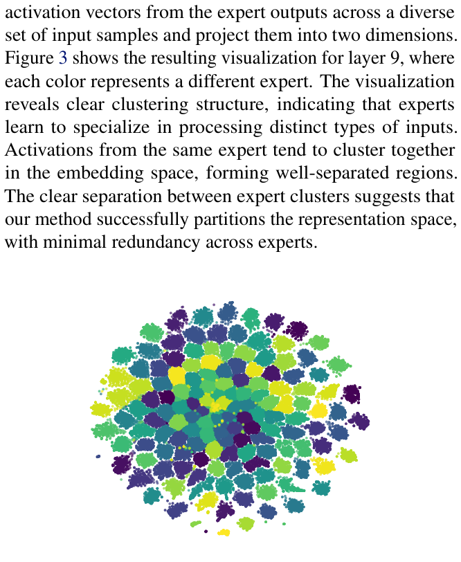
Each color represents a different expert. The clear clustering indicates that experts learn distinct, well-separated representations — without ever being told what to specialize in.
Routing remains well-balanced across all layers:
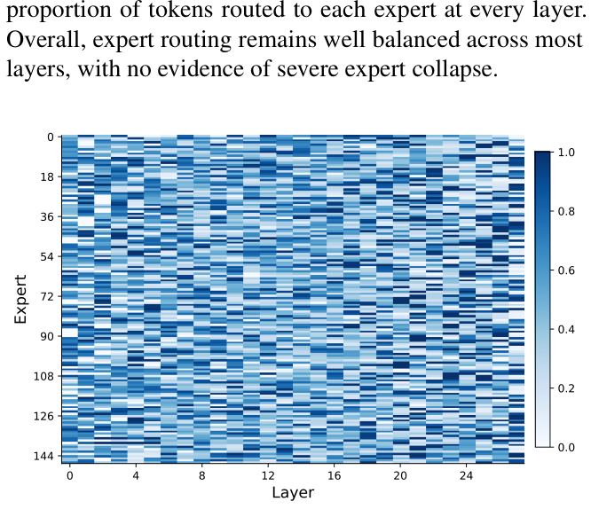
No evidence of severe expert collapse — the load-balancing constraint (combined with the load-balancing loss) keeps utilization roughly uniform.
If you remember nothing else, remember this:
DOT-MoE = Optimal Transport + Sinkhorn + Straight-Through Estimator + Output-Aware Distillation
It converts a pre-trained dense FFN into a sparse MoE by:
A.M_soft.M (forward) while backpropagating through M_soft (STE).W_r with top-k selection (forward hard, backward through softmax via STE).A and W_r end-to-end against a KL-distillation loss from the frozen dense teacher, plus cross-entropy, z-loss, and load-balancing.E real expert FFNs → standard MoE for inference.It beats structured pruning, semi-structured pruning, and every prior dense-to-MoE method (LLaMA-MoE, LLaMA-MoE-v2, CMoE, LTE) across LLaMA-2, LLaMA-3, and Qwen2.5 — retaining 90% of dense performance at 50% active params — and the gains scale (32B) and extend (attention layers, 32K context).
The reason it works: the only signal that matters is the output, and OT+STE is the cleanest way to make a discrete combinatorial assignment learnable end-to-end against that signal.
If you found this useful, clap 👏 and follow for more deep-dives on efficient ML. The DOT-MoE paper is open-access on arXiv — go read it, the appendix is excellent.
Found an error? Have a question? Drop a response below — I read everything.