
Decoupled architecture for real-time vector search in production AI systems
Vector Databases | HNSW | Distributed Systems | 2026
Modern AI systems do not merely store data; they continuously transform raw information into high-dimensional vector representations and must search through them in real time. Every frame of a TikTok video, every transaction in a payment network, every query to a recommendation engine ultimately becomes a point in a 768- or 1536-dimensional vector space. The volume of these vectors is staggering: a single platform processing 380 short-form videos per second, each generating roughly 130 multimodal embeddings across visual, audio, and text modalities, produces approximately 50,000 vectors every single second. That is 4.32 billion vectors per day flowing through a system that must make each one searchable within milliseconds.
The fundamental operation underlying all of this is the K-Nearest Neighbor (KNN) search: given a query vector, find the K most similar vectors in the dataset. Exact KNN, implemented via brute-force comparison against every stored vector, works fine for a few million records. At a billion vectors, however, a single query requires comparing the query against one billion 768-dimensional vectors. The computational cost is enormous:
At 50,000 queries per second, this is not merely slow; it is mathematically impossible with exact methods. The industry answer is approximate nearest neighbor (ANN) algorithms, and the dominant algorithm in production today is Hierarchical Navigable Small World (HNSW).
HNSW is a multi-layered proximity graph. Think of it as a highway system overlaid on a city map. The top layers of the graph are sparse, containing only a small fraction of all vectors connected by long-range edges. These are the expressways: they allow the search algorithm to traverse vast distances across the vector space in just a few hops. The bottom layer, Layer 0, is dense and contains every single vector in the dataset, connected by short-range edges to its immediate neighbors. This is the local street grid, where precise matching happens.
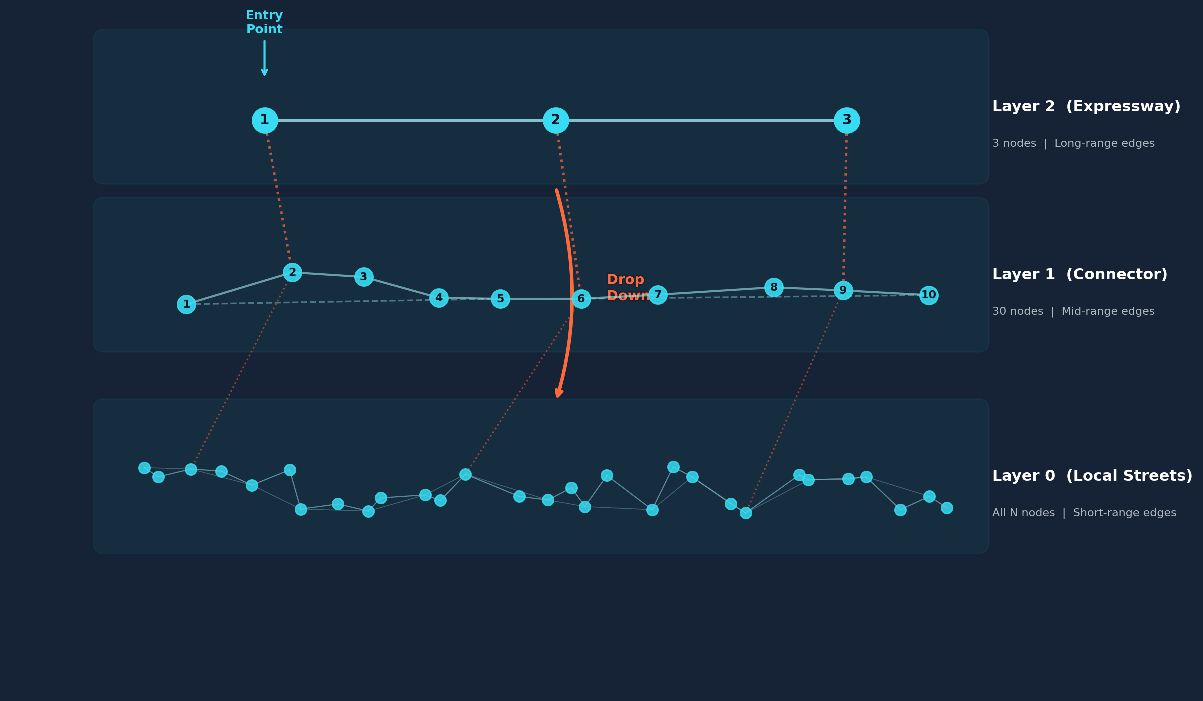
The search algorithm follows a greedy drop-down procedure. It begins at a designated entry point on the highest layer and repeatedly jumps to the neighbor closest to the query vector. When it can no longer find a closer neighbor on the current layer, it drops down to the next layer and repeats the process. Upon reaching Layer 0, the algorithm performs a more exhaustive local search, examining a broader candidate set to find the true nearest neighbors. The critical insight is that each layer acts as a coarse-to-fine filter: the top layers navigate the query into the right neighborhood, and Layer 0 handles the precision work within that neighborhood.
The search complexity of HNSW is:

This is achieved by capping the degree (number of connections per node) at every layer to a constant M, typically between 16 and 64. The logarithmic scaling is handled by the number of layers, not the number of connections. Layer assignment uses an exponentially decaying probability distribution:

This guarantees that Layer 0 contains nearly all vectors, Layer 1 contains roughly 1/M of them, Layer 2 contains roughly 1/M², and so on. The result is a structure mathematically analogous to a skip list, where the expected number of layers grows logarithmically with N.
Why HNSW over the older NSW (Navigable Small World)?
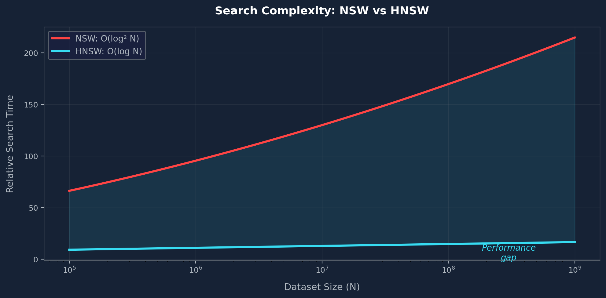
In a flat, single-layer NSW graph, the average degree must grow as O(log N) to keep path lengths short as data grows. This makes the graph a dense, congested hairball with search complexity of O(log² N). HNSW fixes this by capping degree at every layer to a constant M and using multiple layers for the logarithmic scaling instead.
Two parameters govern HNSW behavior. The efConstruction parameter controls write quality: it determines how many candidate neighbors the algorithm examines during insertion. Higher efConstruction produces a better-structured graph with higher recall, but increases the computational cost of each insertion linearly. The efSearch parameter controls read quality: it determines how many candidates the search algorithm tracks during a query. Higher efSearch improves recall at the cost of increased query latency.
In a static, batch-indexed dataset, you can set efConstruction to an aggressive value like 200 or 300 and accept the slow build time. The trouble begins when you try to do this in real time.
There is a fundamental property of HNSW that most tutorials gloss over: insertion is not a simple append operation. To insert a new vector into the graph, the algorithm must first search the graph to find the M closest existing neighbors, then create bidirectional edges to those neighbors. This means every single insertion triggers a full graph search. In a small graph of 10 million vectors, this search might take a few hundred microseconds. In a live production graph with 1 billion vectors, the search for each insertion may require traversing multiple layers and examining thousands of candidate nodes. The cost grows with the size of the existing graph.
Now multiply this by 50,000 insertions per second. Each insertion requires a graph search costing, conservatively, 1 to 5 milliseconds of CPU time:

Even on a 64-core machine, you are consuming 50 out of 64 available cores just on insertion searches, leaving almost no capacity for serving live queries. This is the CPU saturation problem, and it is the first reason why online HNSW indexing fails at this scale.
The second problem is concurrency. HNSW graphs are not inherently thread-safe. When 50,000 insertions are happening simultaneously across multiple threads, they contend for read-write locks on overlapping regions of the graph. Thread A might be searching for neighbors in a cluster while Thread B is inserting a new node and modifying edges in the same cluster. The result is lock contention: threads spend more time waiting for locks than doing useful work, and throughput collapses under Amdahl's law.
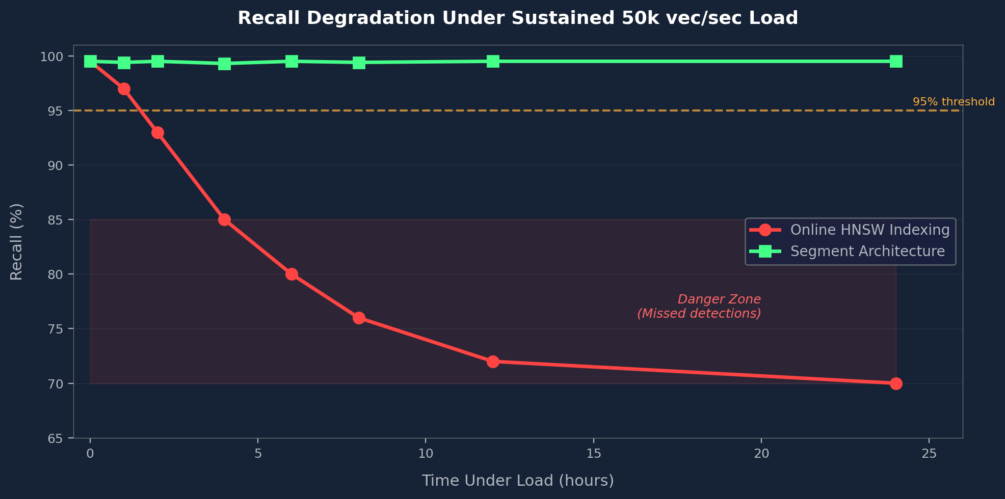
Even more insidious is graph degradation. When insertion pressure is extreme, the algorithm cannot afford to examine enough candidates to find the truly optimal neighbors for each new node. The efConstruction parameter, which might be set to 300 in a batch build, must be reduced to 40 or even 20 in a live system just to keep up with the insertion rate. The consequences are severe: the graph develops structural weaknesses, such as disconnected clusters and poor long-range connectivity.
The Recall Collapse: Recall, the percentage of true nearest neighbors that the algorithm actually returns, drops from the expected 95-99% down to 70-80%. In a copyright enforcement system, that means 20-30% of infringing videos go undetected. In a fraud detection system, that means billions of dollars in missed fraudulent transactions.
The solution to the 50,000 vectors per second bottleneck is not a better graph algorithm. It is a better architecture. The fundamental insight is to decouple data ingestion from graph construction. Instead of inserting vectors one at a time into a live, query-serving graph, the system separates the problem into two independent phases that can be optimized separately.
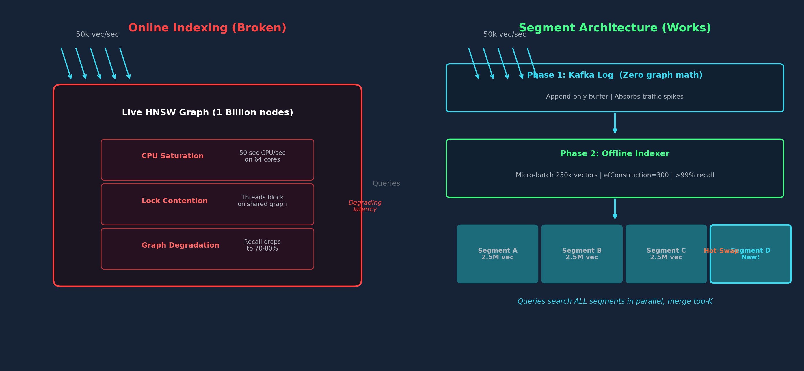
During Phase 1, incoming vectors are appended to an unindexed, append-only log. This is typically implemented using Apache Kafka or a similar distributed message broker acting as a shock absorber. The key property of this phase is that absolutely zero graph construction mathematics happens here. The system is simply writing vectors to a durable log, an operation that can handle hundreds of thousands of vectors per second on modest hardware.
Kafka also provides the critical ability to buffer traffic spikes: if a burst of 200,000 vectors arrives in a single second, the message queue absorbs the shock and delivers them to downstream consumers at a rate they can handle, preventing system-wide cascading failures. This is the "shock absorber" pattern that makes the architecture resilient to real-world traffic variability.
In Phase 2, a pool of CPU indexer pods consumes vectors from the log and accumulates them into micro-batches. When a batch reaches a target size, typically 250,000 vectors, the indexer builds a completely isolated HNSW graph, called a segment, using an aggressive efConstruction value of 200 to 300. Because this construction happens offline, on a batch that is not serving any live queries, the indexer can take as much time as it needs to find the mathematically optimal position for every node.
Why this works: There are no lock contention issues because the segment is built in a single-threaded or partition-locked context. There are no latency constraints because no user is waiting for this specific segment to be built. The result is a compact, highly optimized HNSW graph that achieves greater than 99% recall.
Once built, the segment is serialized to a binary format and uploaded to object storage, such as AWS S3, from where it can be loaded into the RAM of the vector database's query nodes.
The final piece of the architecture is the hot-swap. When a new segment is ready, the vector database's query nodes download it from object storage, load it into RAM, and update their internal routing table to include the new segment in future queries. This swap is atomic from the perspective of the query path: a query that begins before the swap completes searches the old set of segments, and a query that begins after the swap searches the new set. There is no downtime, no query disruption, and no performance degradation during the transition. Within seconds of a segment being built, its vectors are fully searchable alongside all previously built segments.
Putting all of this together, the complete production pipeline for handling 50,000 vectors per second consists of five stages, each running as an independently scalable microservice:
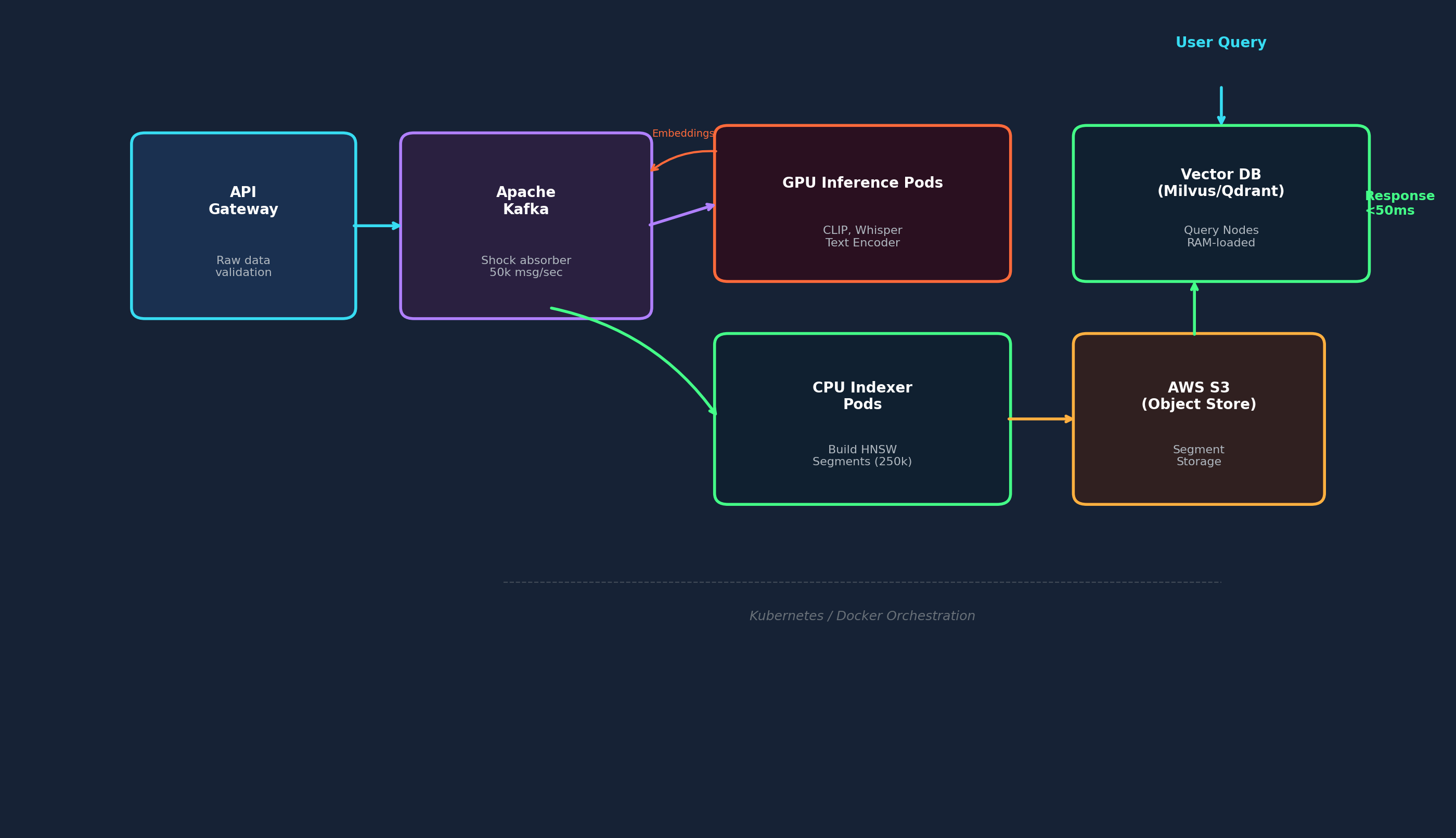
Stage 1 — API Gateway: Receives raw data from upstream sources such as video uploads or transaction events, validates the payload, and publishes it to the first Kafka topic. The gateway is stateless and horizontally scalable, capable of absorbing arbitrary traffic spikes behind a load balancer.
Stage 2 — GPU Inference Pods: A pool of Docker containers orchestrated by Kubernetes. These pods consume raw data from Kafka, run heavy AI models to generate vector embeddings, and publish the resulting vectors to a second Kafka topic. For a video moderation system, this means running CLIP for visual embeddings, Whisper for audio embeddings, and a text encoder for caption or title embeddings. The GPU pool scales independently based on queue depth: more traffic means more GPU pods are spun up automatically.
Stage 3 — CPU Indexer Pods: A separate pool of CPU-only pods consumes the embedding vectors from the second Kafka topic, accumulates them into micro-batches of 250,000, and builds the offline HNSW segments. Each indexer pod operates on its own partition of the Kafka topic, so there is no cross-pod coordination needed. The completed segment files are uploaded to S3.
Stage 4 — Object Storage (AWS S3): Provides durable, highly available backing store for all segment files. This ensures the system can recover from node failures without data loss and enables any query node to download any segment on demand.
Stage 5 — Vector Database (Milvus / Qdrant / Weaviate): Query nodes monitor S3 for new segment files. When a new segment appears, a query node downloads it, loads it into memory, and begins routing queries to it. The entire query path, from receiving a user query to returning top-K results, operates in under 50 milliseconds.
| Stage | Component | Role | Scaling |
|---|---|---|---|
| 1 | API Gateway | Receive, validate, buffer | Horizontal (stateless) |
| 2 | Kafka | Shock absorber / message queue | Partition-based |
| 3 | GPU Inference Pods | Generate vector embeddings | HPA (queue depth) |
| 4 | CPU Indexer Pods | Build HNSW segments offline | Per-partition parallelism |
| 5 | Object Storage (S3) | Durable segment storage | Virtually unlimited |
| 6 | Vector DB Query Nodes | Serve user queries <50ms | Shard-based |
Consider a TikTok-scale short-form video platform. The platform processes 380 video uploads per second. Each video, typically 15 to 60 seconds long, is segmented into keyframes and audio windows. A CLIP model generates visual embeddings for each keyframe, a Whisper model generates audio embeddings for each audio window, and a text encoder processes the video title, description, and any overlaid text. A typical video generates approximately 130 vector embeddings across these three modalities.
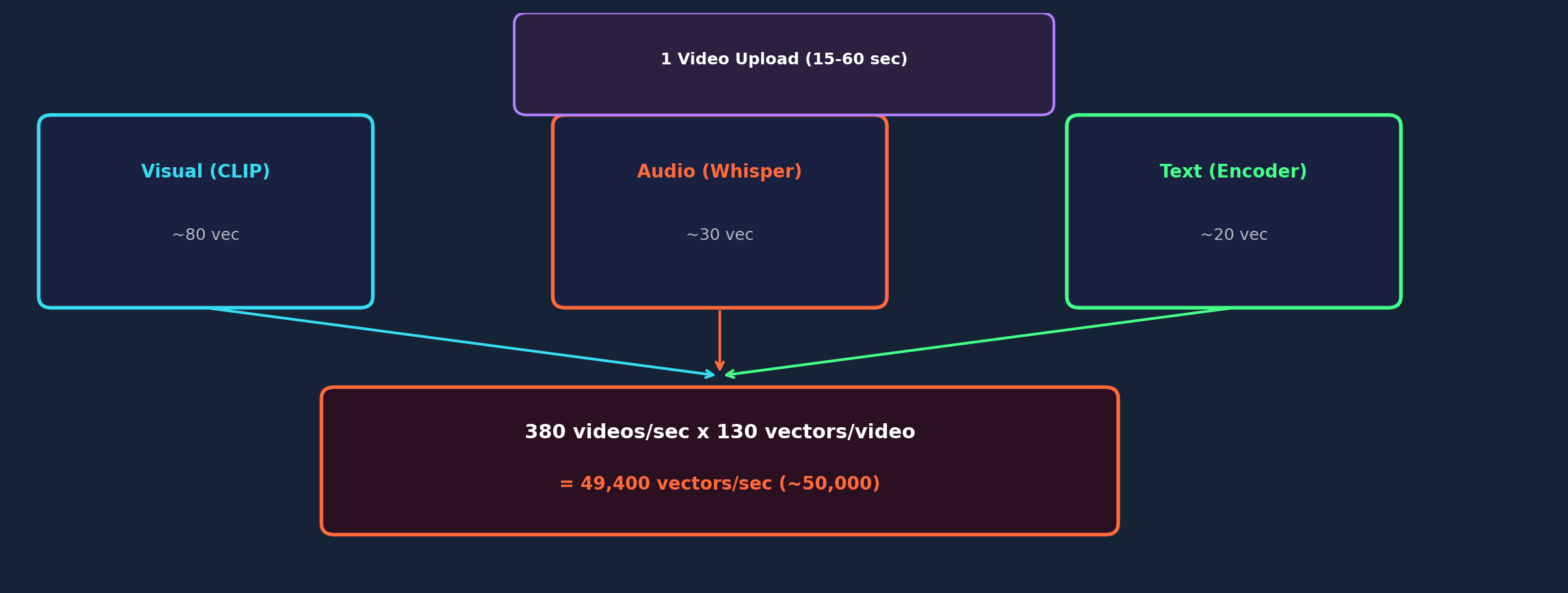
The math is straightforward:

The system must search these vectors against a reference database containing billions of known copyrighted content vectors to detect infringement, and simultaneously route each video to the appropriate recommendation cluster based on its semantic similarity to existing content categories. Both operations require sub-50-millisecond latency to meet real-time processing requirements.
Why online indexing fails here: If this system attempted online HNSW indexing, the insertion load would degrade the graph within minutes. Recall would drop below 80%, meaning roughly one in five infringing videos would slip through undetected. Copyright holders would notice, legal liability would accumulate, and the platform would face regulatory consequences.
The segment-based architecture eliminates this problem entirely. Ingestion absorbs the 50,000 vectors per second into Kafka without any graph computation. Offline indexers build high-quality segments with efConstruction of 300, achieving greater than 99% recall. The hot-swap mechanism makes each batch searchable within seconds, ensuring that even newly uploaded infringing content is detected within a narrow time window.
As the system operates over weeks and months, it naturally accumulates many small segments. A naive approach would let the segment count grow without bound, but this creates a query performance problem: a search query must examine every active segment in parallel, collect the top-K results from each, and merge them into a final result set. If the system has 1,000 segments, each query fans out to 1,000 parallel searches, creating massive CPU overhead and I/O contention.
The solution is compaction. A background offline job periodically merges small segments into larger ones:

The merge process rebuilds a fresh HNSW graph over the combined vectors, maintaining the same high efConstruction quality. This strictly bounds the total number of active segments to roughly 20 to 100 at any given time, regardless of how long the system has been running or how many vectors have been ingested.
For trillion-scale deployments, the system adds horizontal sharding. The vector space is partitioned across multiple physical machines using a consistent hashing or range-partitioning scheme. A load balancer examines each query and routes it only to the shard or shards that hold the relevant partition of the vector space. This ensures that each shard handles only a fraction of the total data, keeping query latency constant even as the total dataset grows.
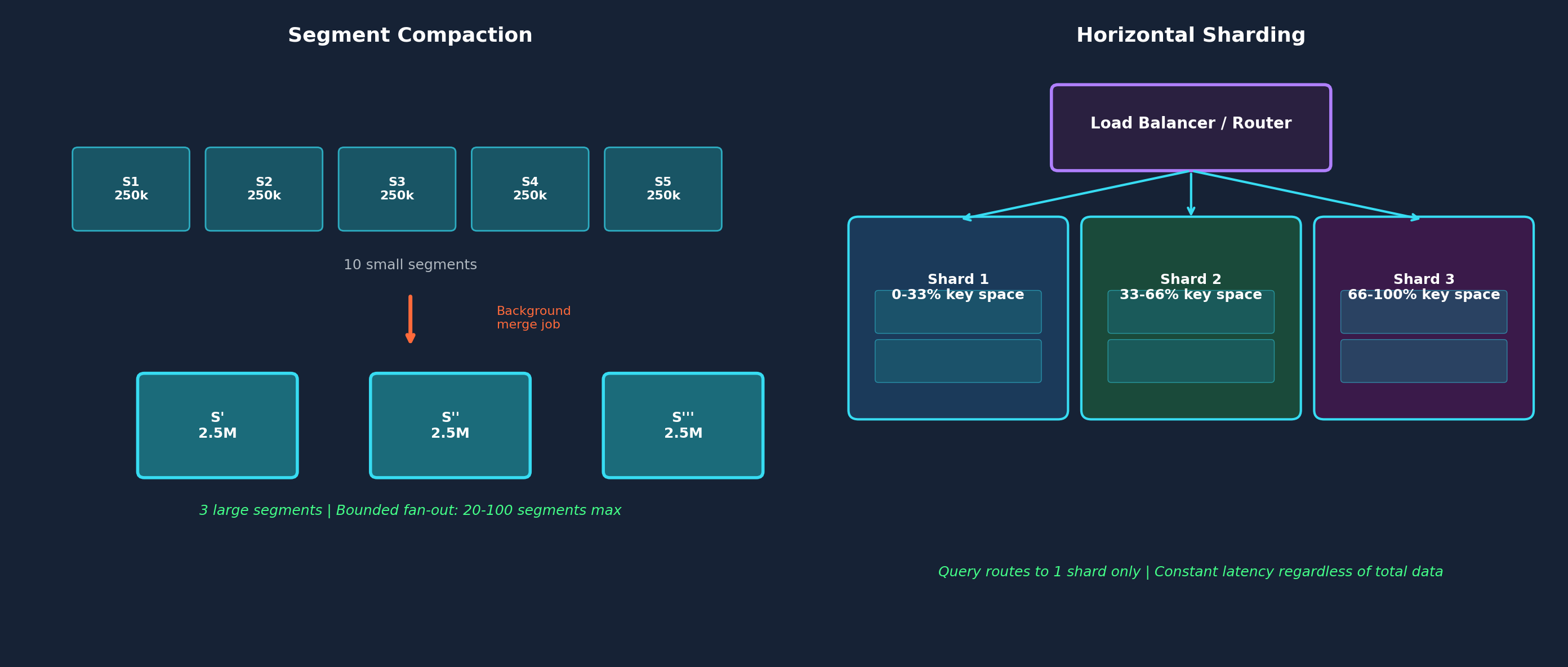
Sharding and compaction together provide the theoretical foundation for infinite scalability: the system can handle any data volume by adding more shards, while compaction prevents query fan-out from growing unboundedly within each shard.
The 50,000 vectors per second bottleneck is not a failure of the HNSW algorithm. HNSW is, by every metric, the best approximate nearest neighbor algorithm available today. The failure is architectural: trying to use a batch-optimized algorithm in a streaming context without adapting the surrounding system.
The segment-based architecture described in this article applies a classic engineering principle: decompose an intractable problem into tractable sub-problems. By decoupling ingestion from indexing, the system achieves both the throughput of a simple log append and the recall quality of a carefully constructed graph. Each component — Kafka, GPU inference, CPU indexing, object storage, and the vector database — operates independently and can be scaled, upgraded, or replaced without affecting the others.
This pattern, decoupling the hot path from the cold path, appears repeatedly in distributed systems design. Search engines build index segments offline and serve them online. Database systems separate write-ahead logs from LSM tree compaction. Stream processing frameworks batch micro-batches before committing to state stores. The segment architecture for vector search is the same principle applied to the specific constraints of high-throughput approximate nearest neighbor search.
If your system ingests fewer than a few thousand vectors per second, a single online HNSW graph is perfectly adequate. But the moment you cross the threshold where insertion cost begins to degrade graph quality, decoupling is not merely an optimization. It is the only architecture that works.